The two analyzed studies found that, despite different methodologies and subjects, phase-amplitude coupling is increased in advanced stages of the disease. However, variability in the findings during different activities (motor tasks vs. sleep) and different stages of the disease suggests that the underlying mechanisms leading to increased phase-amplitude coupling in Parkinson’s disease are not yet fully understood. Consequently, employing phase-amplitude coupling as a control signal in adaptive deep brain stimulation therapy might be considered premature.
Summarizing statement
Deep brain stimulation is a neurosurgical treatment for Parkinson’s disease to alleviate motor symptoms such as tremor, rigidity, and akinesia. In an attempt to improve this therapy, research suggests using measures of phase-amplitude coupling (a form of synchronization between different neural oscillations) as a control signal for deep brain stimulation therapy. The aim of this paper is to compare two studies with regard to the purported role of phase-amplitude coupling in Parkinson’s disease and deep brain stimulation therapy. The paper provides a brief introduction to Parkinson’s disease and cross-frequency coupling, in particular phase-amplitude coupling. It then analyzes the two studies mentioned above in terms of their methodology and results. It concludes with a short summary and further research questions
The adaptive exponential integrate-and-fire model is a simple yet powerful model for describing neural activity. It is capable of modeling a wide range of firing patterns observed experimentally. We attempt to answer the question of how the dynamics of the model give rise to different firing patterns and discuss its biophysical realism when matched against experimental data. We provide a computational implementation1 using the Julia programming language. Our results suggest that the chosen environment is well-suited for simulating neuronal activity.
1. Introduction
Neurons are considered the basic information processing units of the nervous system. Understanding how they encode and process information is therefore a fundamental research area in neuroscience. Neurons interact primarily2 with all-or-none electrical signals, named action potentials or spikes. The discovery of how voltage-gated ion channels generate action potentials is a part of the Nobel Prize-winning legacy of Hodgkin and Huxley (1952). They described the membrane voltage as a function of currents that pass through ion channels in the cell membrane, allowing the formulation of a theoretical mathematical model to describe and to computationally simulate neuronal activity (Hodgkin and Huxley, 1952). Models that incorporate these biophysical details are accordingly referred to as Hodgkin-Huxley-type models. However, while Hodgkin and Huxley described the electrophysiology of the giant squid axon, neuronal models have become increasingly complex to account for the rich biophysics of the different types of ion channels observed in vertebrate nervous system neurons. Detailed biophysical models are able to reproduce experimental electrophysiological data with high accuracy but, due to their complexity, are difficult to analyze and computationally expensive. This complexity becomes a limitation when scaling networks of spiking neurons for analyzing the behavior of neural systems. Therefore, mathematically simpler neuron models are widely used in studies of neural coding, memory, and network dynamics (Gestner et al., 2014, ch. 5). Models that describe the membrane voltage only as a function of input current to predict spike times, without accounting for the biophysical mechanisms (such as ionic currents) that underlie the initiation of an action potential, are called integrate-and-fire models.
The idea behind integrate-and-fire models remarkably tracks back to Lapicque (1907), long before Hodgkin and Huxley discovered the mechanisms responsible for the generation of action potentials (Abbott, 1999). Integrate-and-fire models have two fundamental components: an equation that describes the evolution of the membrane potential and a mechanism to generate spikes. A simple and widely used version is the leaky integrate-and-fire (LIF) model. The adaptive exponential integrate-and-fire (AdEx) model introduced by Brette and Gerstner (2005) extends more basic integrate-and-fire models to incorporate more biophysical realism.
In this paper, we provide a complete description of the AdEx model and analyze the underlying mathematical equations with emphasis on the system's dynamics that give rise to different firing patterns. We conclude the theoretical part by discussing the derived properties in contrast to other integrate-and-fire models. Finally, we present a computational implementation of the AdEx model within the Julia programming language (Bezanson et al., 2017).
2. Background
In this section, we derive the AdEx model by using the LIF model as a starting point before discussing the model itself. First, we want to introduce some key terms that might aid in gaining a better intuition for integrate-and-fire models. In analogy to a simple resistor–capacitor electric circuit, the cell membrane represents the capacitor that provides electrical insulation between the intra- and extracellular fluid. It accumulates electrical charge and can integrate inputs from external sources. The membrane potential refers to the voltage difference across the membrane. The membrane capacitance is proportional to the cell surface area and determines how much current flow is required to change the membrane potential. However, the membrane is not a perfect insulator, so that ions flow (leak) across the membrane. The leak conductance is inverse to the membrane resistance and determines how easily ions flow across the membrane. The development of the membrane potential over time is mathematically described by a differential equation. Other parameters can also functionally evolve with time.
2.1. Integrate-and-fire models and adaptation
The LIF model is defined by a linear differential equation that describes the dynamics of the membrane potential (\(V \)) of a neuron as it integrates an incoming current (\(I \)) and leaks charge over time (Izhikevich, 2007):
\[(1) C\dfrac{dv}{dt} = -g_{L}(V - E_{L}) + 1 \]
\(C \) denotes the membrane capacitance, \(g_{L} \) the leak conductance, \(E_{L} \) the leak reversal potential and \(I \) is the synaptic current. The term \(V - E_{L} \) is often referred to as the driving force. When the membrane potential reaches a threshold, the neuron generates a spike and is set back to a reset potential. The leak term \(-g_{L}(V - E_{L}) \) reflects the diffusion of ions through the membrane. The input \(I \) is integrated linearly and independently of the neuron's state, so the LIF model has no memory of its previous spiking behavior. This model turns out to be insufficient to account for the electrophysiological characteristics of actual neurons.
In order to make the model biophysically more realistic, first, the spike generation mechanism needs to be adjusted. Instead of generating a spike when the membrane potential reaches a threshold, a nonlinearity is introduced to account for the upswing of an action potential. The upswing is stopped at a reset condition. Fourcaud-Trocmé et al. (2003) proposed the exponential integrate-and-fire (EIF) model and have shown that near the threshold, the sodium activation variable in a Hodgkin-Huxley-type model can be well approximated by an exponential function:
\(V_{T} \) denotes the threshold and \( Δ_{T} \) the slope factor responsible for the sharpness of an action potential.
The second adjustment concerns the lack of memory. Brette and Gerstner (2005) proposed an integrate-and-fire model with adaptation, called the AdEx model. The model is extended by the introduction of an adaptation variable \(ω \), which changes depending on the membrane potential. Moreover, \(ω \) is incremented by a fixed value if the reset condition is triggered, i.e., the neuron spikes, thus adding a mechanism to remember previous events. The adaption variable \(ω \) is then incorporated into the equation (2):
The adaptation mechanism is introduced by adding a second equation to the model, i.e., making it two-dimensional.
\[(4) τ_{ω}\dfrac{dω}{dt} = a(V - E{L} - ω) \]
Here, \(τ_{ω} \) is the adaptation time constant and \(a \) is a constant controlling the adaptation. By including the exponential nonlinearity and the adaptation mechanism, the LIF model has been transformed into the AdEx model.
Another important model related to the AdEx model was proposed by Izhikevich (2003). The Izhikevich model has dimensionless variables and is therefore more abstract compared to the AdEx model. Both models are two-dimensional and share the adaptation mechanism. Instead of the leak term and the exponential nonlinearity, the Izhikevich model uses a quadratic function. We will briefly discuss the differences between the Izhikevich and the AdEx model in section 5.
2.2 Adaptive exponential integrate-and-fire model
Having established the two equations of the AdEx model, 3 and 4, we can further discuss the components of the model, originally proposed by Brette and Gerstner (2005).
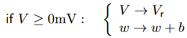
The membrane potential \(C \) evolves over time according to equation (3). The capacitive current \(C\dfrac{dV}{dt} \) is balanced by the injected current \(I \) and the negative of the leak current and exponential term. The leak current \(g_{L}(V - E_{L}) \) is linear in the membrane potential \(V \) and increases as \(V \) rises above the leak reversal or resting potential \(E_{L} \). The leak conductance \(g_{L} \) and resting potential \(E_{L} \) determine the passive leakiness of the membrane. These parameters influence how the membrane potential decays towards the resting potential in the absence of input currents. The exponential term is close to zero at rest and increases rapidly when \(V \) crosses the spike threshold \(V_{T} \). The spike threshold \(V_{T} \) and the slope factor \(δ_{T} \) influence the sharpness of the spike initiation process. A lower threshold or a steeper slope leads to more rapid spiking in response to input currents. Mathematically, \(V \) diverges towards infinity when the neuron spikes. In practice, the upswing is stopped at the reset condition, which is triggered when \(V > 0mV \). The downswing is not described by the differential equation but by the reset condition
Equation (5)
with reset potential \(V_{r} \) and spike-triggered adaptation \(b \). Usually, the trigger voltage for the reset condition would be set to 20 mV for most neurons in physiological conditions. Due to the nature of the exponential nonlinearity, the upswing of the action potential is rather steep, well above the threshold potential (\(V_{T} \)), so using a reduced trigger voltage (e.g., 20 mV) has no significant influence on spike timing. The trigger voltage can, however, affect numerical simulations (see section 4). (Brette & Gerstner, 2005)
The adaptation variable \(ω \) is governed by equation 4 with time constant \(ω_{τ} \). The adaptation variable introduces a feedback mechanism as described in the previous section. Assuming \(b > 0 \), due to the spike-triggered adaptation mechanism, \(ω \) increases as the membrane potential approaches the threshold. This increase in \(ω \) then contributes to a decreasing firing rate over time. Note that the opposite effect can also be achieved if the parameters are set to \(b = 0 \) and \(a < 0 \). (Brette & Gerstner, 2005)
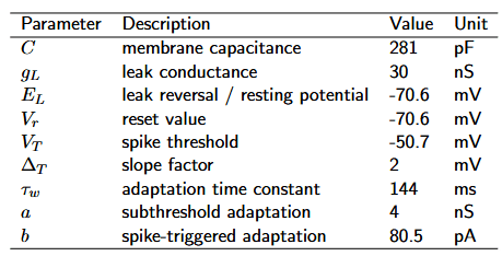
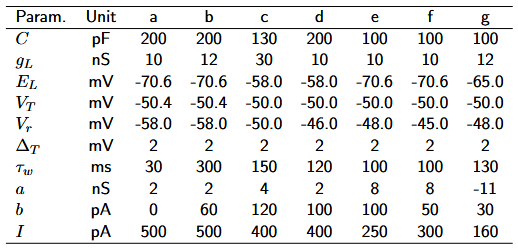
As a reference, an overview of the parameters is given in Table 1.
Table 1: Parameter description for the AdEx model. The parameter values are taken from the original paper (Brette & Gerstner, 2005), modeled after regular spiking pyramidal cells.
3. Model analysis
In this section, we will investigate the AdEx model in order to understand its electrophysiological features. The dynamics can best be described by a phase plan analysis. We discuss how the model’s dynamics give rise to different firing patterns.
3.1 Phase plane analysis
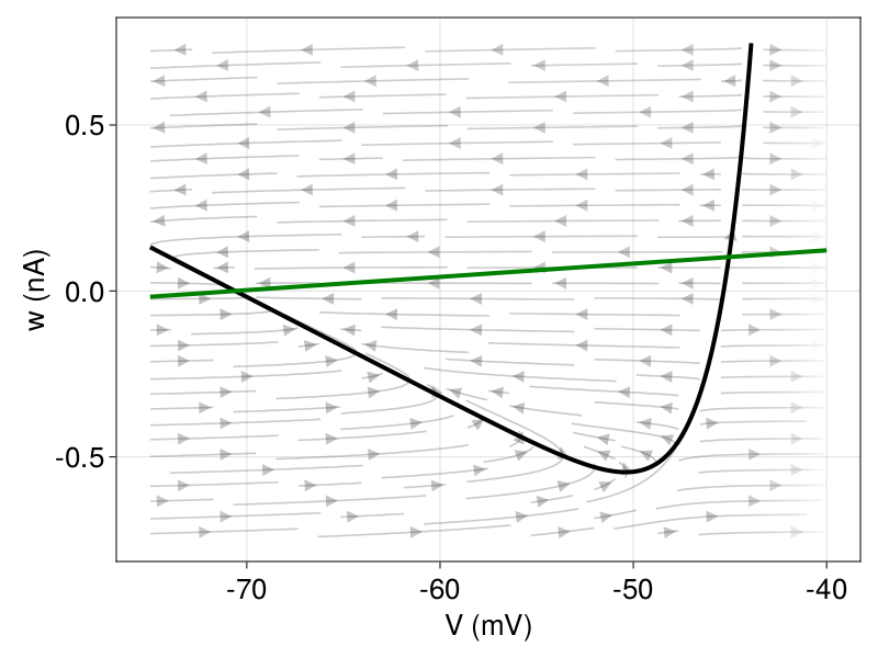
Phase plane analysis offers insights into the dynamics of the AdEx model. To visualize the behavior of the system, we plot the vector field and the nullclines \(\dfrac{dV}{dt} = 0 \) (V-nullcline) and \(\dfrac{dω}{dt} = 0 \) (ω-nullcline).
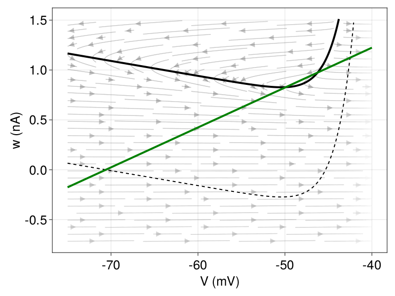
Figure 1: Phase plane with indication of the vector field, V-nullcline (black) and w-nullcline (green). Left In absence of an input current (\( I = 0 \)), there is a stable fixed point at 70.6 mV (resting potential) and an unstable fixed point above the spike threshold. Right Andronov-Hopf bifurcation: After current injection (black), the stable fixed point loses stability before the two fixed points merge.
The dynamics are characterized by the number and the type of fixed points, which are the intersections of the two nullclines. As the \(V \)-nullcline is a convex function, characterized by the exponential term, the maximum number of fixed points is two. Figure 1 (left) shows the phase plane in the absence of an input current, i.e., \(I = 0 \), given the parameters in Table 1. We have a stable fixed point at \(E_{L} \) and an unstable fixed point above the spike threshold (\(V_{T} \)). When a sufficient input current is applied, i.e., \(I \) increases, the V-nullcline shifts up and the stable fixed point loses stability. This critical current \(I \), at which the transition from the resting state to spiking occurs, is called the rheobase3. The sudden change in the behavior of the dynamical system (from resting to spiking) is mathematically referred to as a bifurcation. The rheobase current depends on the type of bifurcation. In the AdEx model, the choice of parameters \(a \) and \(τ_{ω} \) determines whether the loss of stability is via an Andronov-Hopf or via a saddle-node bifurcation (Figure 1, right). To simplify the classification, we introduce a time scale variable \(τ_{m} = \dfrac{C}{g_{L}} \). The stable fix point becomes unstable through an Andronov-Hopf bifurcation if \(\dfrac{a}{g_{L}} > \dfrac{τ_{m}}{τ_{ω}} \) (Touboul, 2008). Otherwise, there is a saddle-node bifurcation where both fixed points merge and disappear.
The type of bifurcation has no influence on the firing pattern, but on the subthreshold dynamics. Along with an additional condition, the bifurcation type influences the occurrence (resonator) or absence of subthreshold oscillations (integrator). Considering inputs of multiple pulses (e.g., bursts), the model will show a different behavior depending on whether it acts as an integrator or a resonator. The response of a resonator depends on the input frequency in relation to the damped oscillation. For a complete classification of the dynamics and bifurcations, we refer to Touboul (2008).
3.2 Firing patterns
The type of firing pattern generated by the AdEx model depends primarily on the choice of subthreshold adaptation \(a \) and reset parameters (reset value \(V_{r} \) and spike-triggered adaptation \(b \)). We will look at six different firing patterns and explain them based on the dynamics in phase space. All simulations were run for 300 ms, injecting a (constant) step current from 50 ms to 250 ms. The underlying parameters are provided in Table 2.
3.2.1 Tonic and adapting firing patterns
The simplest type of spiking pattern is a regularly spaced discharge of action potentials called tonic firing (Figure 2). A tonic firing can also be produced by a LIF model with a constant current supply. The AdEx model exhibits a tonic pattern when the sensitivity to subthreshold voltage changes is small (subthreshold adaptation \(a \) small or \(τ_{ω} \) high) and in the absence of spike-triggered adaptation (\(b = 0 \)). The \(ω \)-nullcline is almost flat. \(ω \) increases only marginally despite high-frequency spiking.
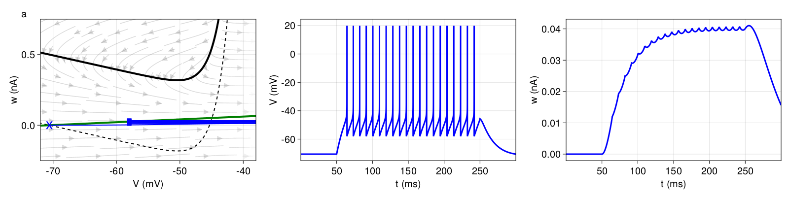
Figure 2:Tonic spiking (pattern a). Left Phase plane with V-nullcline (black), V-nullcline at \(I = 0 \) (dotted), ω-nullcline (green) and trajectories (blue). The blue cross marks the resting state and the blue squares the resets according to equation 5. For better illustration, the trajectories shown in the phase plane are clipped after some resets, depending on the pattern. Middle<\b> Firing pattern (state variable \(V \), equation \eqref{eq:adeif}). Right Adaptation pattern (state variable \(ω \), equation 4).
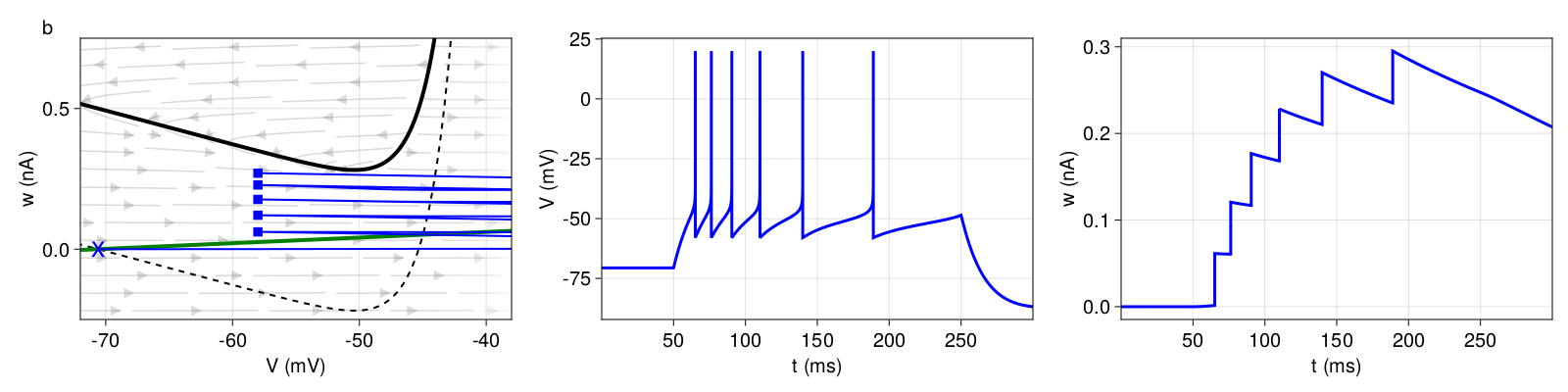
Figure 3:Adaptation (pattern b). Structure and coloring conventions as in Figure 2.
Adaptation leads to a gradual increase (or decrease) in the inter-spike intervals. In Figure 3, we observe the effect of the spike-triggered adaptation \(b > 0 \) and a slow adaptation (\(τ_{ω} = 300ms \). As long as the reset lands below the \(V \)-nullcline, the membrane potential increases immediately after reset, but with decreasing velocity as \(ω \) builds up towards the \(V \)-nullcline. This leads to a prolongation of the refractory period.
3.2.2 Bursting
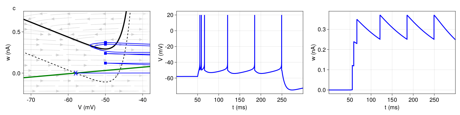
In Figure 4 (top), we observe a short initial burst and a regular spiking behavior afterwards (tonic spiking). With every reset, ω is shifted upwards by \(b = 120pA \). On closer inspection, the initial burst exhibits gradually increasing inter-spike intervals (adaptation) but at high frequency. The high frequency is primarily caused by the reset value \(V_{r} \) equal to the threshold \(V_{T} \). After the third spike, the landing point (after reset) is above the \(V \)-nullcline, initiating a prolonged refractory period. This is called a detour reset. The system then settles into a regular spiking behavior. During the refractory period, \(ω \) decreases only enough for \(b \) to shift the next landing point again above the \(V \)-nullcline (again, detour reset).
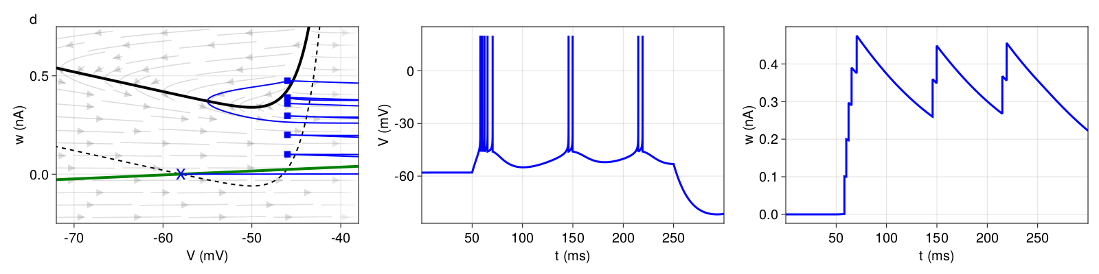
Figure 4: Top: Initial bursting (pattern c). Bottom: Regular bursting (pattern d). Structure and coloring conventions as in Figure 2.
With the more regular bursting pattern in Figure 4 (bottom), the phase plane looks almost identical. But instead of regular spiking behavior after the initial burst, we repeatedly observe two-spike bursts. Here, the parameters are only slightly different. But, after each extended refractory period (detour reset), the increase in ω is sufficiently small that the next landing point is below (rather than above) the \(V \)-nullcline. As a result, the system generates an immediate second spike before the next detour reset.
3.2.3 Transient spiking
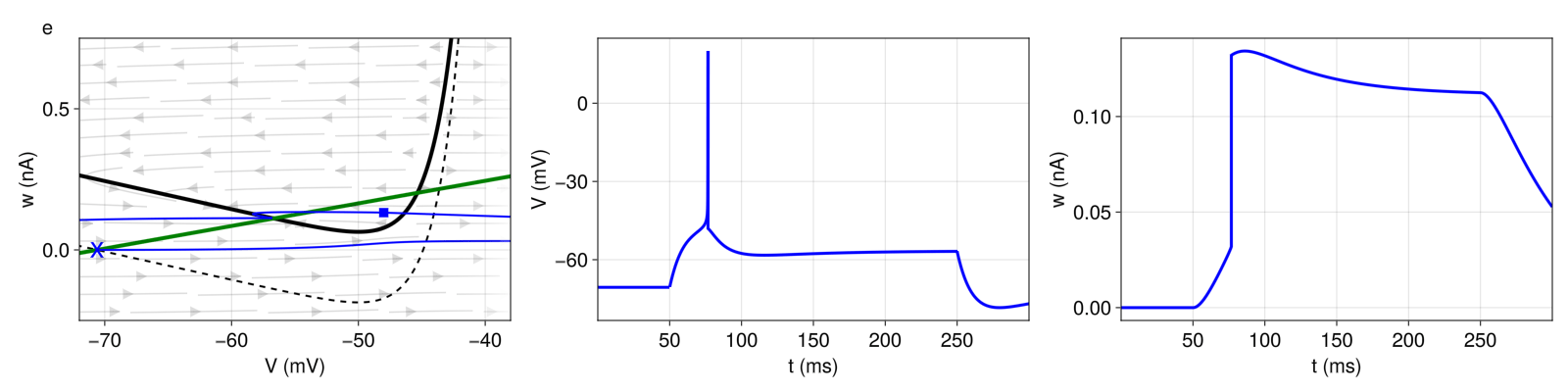
If a neuron only fires a single spike or a short burst and then remains silent despite constant current injection, we speak of transient or phasic spiking behavior (Figure 5). The key difference to non-transient patterns is that the two nullclines intersect even when the external current is applied, so that a stable fixed point remains. In other words, the input current is not sufficient to destabilize the stable fixed point. The upswing that leads to an action potential is due to a sudden increase in the current (here: below the rheobase). If we were to increase the current gradually, the neuron would not fire because our system would remain in the attraction basin of the stable fixed point. Here, the transient spiking behavior is caused by high subthreshold adaptation (\(a = 8nS \)), which increases the slope of the w-nullcline and leads existence of a stable fixed point. During the upswing, ω increases high enough for the landing point to be above the \(V \)-nullcline and in the basin of attraction of the stable fixed point, where the system converges with the stimulus still applied.
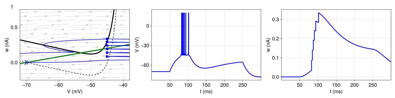
Figure 5: Top: Transient spiking (pattern e). Bottom: Transient bursting (pattern f). Structure and coloring conventions as in Figure 2.
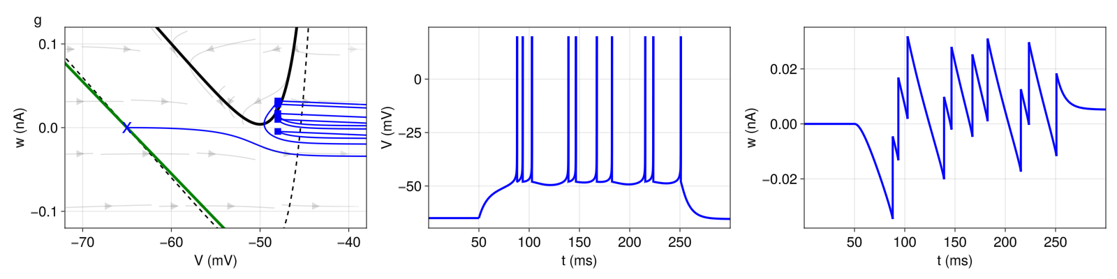
Figure 6: Irregular spiking pattern (pattern g). For better readability, the trajectory in the phase plane (left) is only shown for the first five resets. Structure and coloring conventions as in Figure 2.
For transient bursting, we set the same subthreshold adaptation \(a \), hence obtain a stable fixed point even with external current input, but increase the reset value \(V_{r} \) slightly, so that the first landing points are outside of the attraction basin of the stable fixed point. The bursting mechanism is the same as before. With every reset, ω is shifted upwards by \(b = 100pA \) until a landing point crosses the \(V \)-nullcline. Here, this last reset is a detour reset followed by a prolonged refractory period, after which the system will converge at the stable fixed point.
3.2.4 Irregular firing patterns
Figure 6 exhibits an irregular firing pattern. This pattern is primarily generated by the choice of subthreshold adaptation \(a < 0 \) and spike-triggered adaptation \(b > 0 \). The model switches irregularly between direct resets (landing point below the \(V \)-nullcline) and detour resets (above the \(V \)-nullcline), thus inducing the irregular pattern.
Table 2: Parameter for the six different firing pattern (a-g) in Figures 2 to 6. The firing patterns are mostly adopted from Naud et al., 2008).
3.3. Parameter space
On the basis of the observations made in the previous section, we can now examine how different parameter configurations give rise to different firing patterns. Following the procedure by Naud et al., 2008), we conduct a grid classification to approximate the parameter space. To reduce the dimensionality of the parameter space, we fix parameters that have no influence on the firing pattern (\(C = 200pF \), \(g_{L} = 10nS \), \(E_{L} = -70mV \), \(V_{T} = -50mV \) and \(Δ_{T} = 2mV \)). As previously discussed, transient and non-transient patterns have different configurations in terms of the subthreshold adaptation \(a \) and the input current \(I \). All simulations were run for 100 ms, injecting a constant step current from 10 ms to 90 ms.
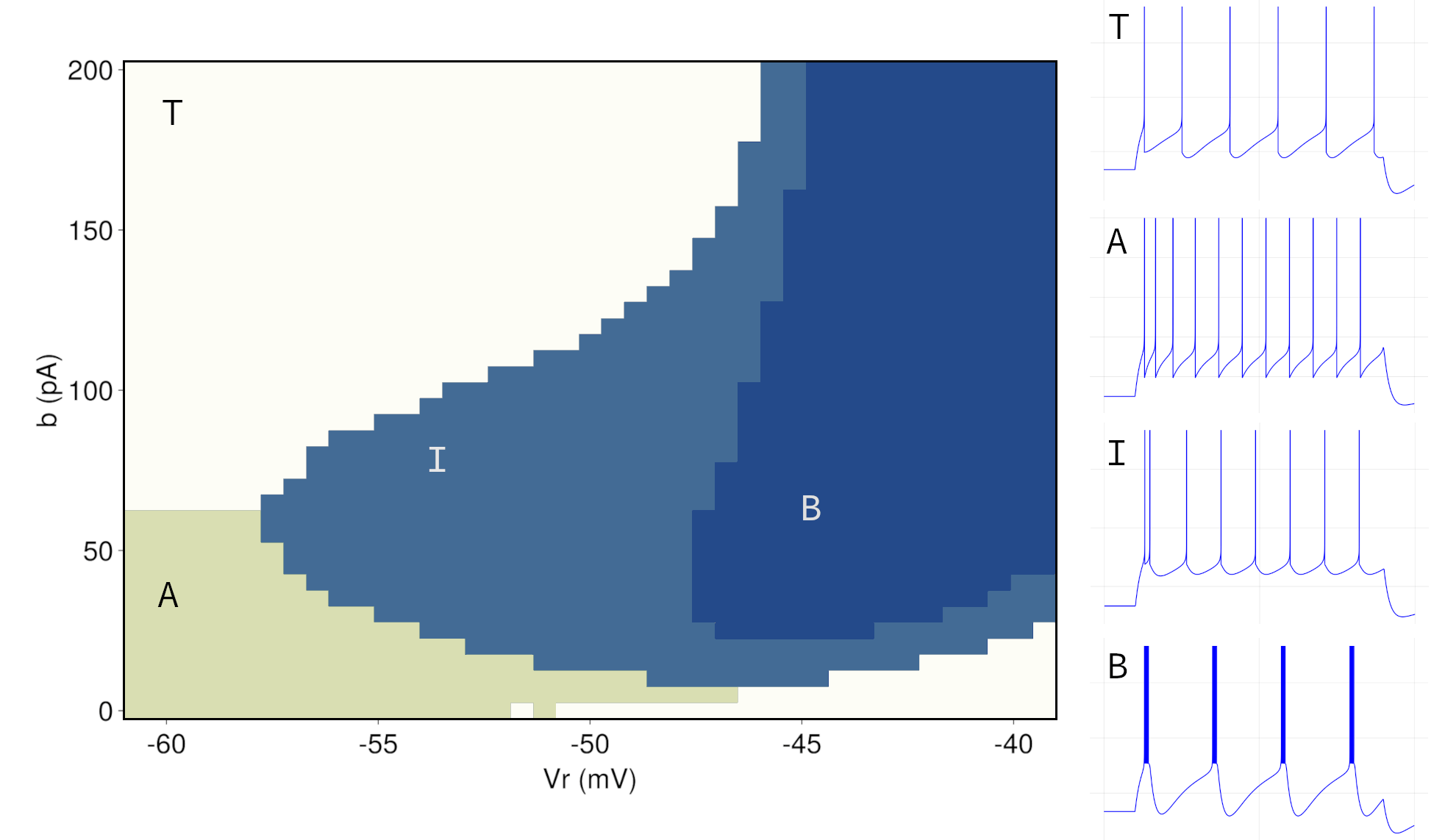
For non-transient patterns, we choose the input current well above rheobase. In order to allow for some adaptation, we set the adaptation time constant \(τ_{ω} = 100 ms \) and subthreshold adaptation \(a = 2nS \). The parameter space is then obtained via numerical simulation for our grid parameters, the reset value \(V_{r} \) and the spike-triggered adaptation \(b \). To automate the process, we use an algorithm to discriminate between the different firing patterns. Since we allow for adaptation, tonic firing only has to take place after the second spike. This approach is consistent with the literature (Naud et al., 2008) and ensures comparability of the results. Bursts are identified statistically based on inter-spike times. Well above the rheobase current, tonic and adapting firing as well as bursting patterns occupy most of the parameter space. Irregular firing patterns mostly occur with parameters close to those of the regular bursting patterns, but are in general rather difficult to pinpoint in the parameter space. Figure 7 shows the results of the grid classification and the partition of the parameter space for tonic (T), adapting firing (A), as well as initial (I) and regular (B) bursting patterns. Irregular firing patterns, as mentioned, occur in the vicinity of regular bursting patterns, but are not displayed due to their sparse nature and the chosen grid resolution. At the transitions between different patterns in the parameter space, differences are often undetectable by visual inspection, so inter-spike statistics are required to obtain boundaries in the parameter space. Tonic patterns in the upper left (area T) exhibit constant length refractory periods after the second spike. The combination of a rather high spike-triggered adaptation \(b \) and low reset value \(V_{r} \) leads to a balance in the adaptation variable \(ω \), where the change in \(ω \) during refractory is nearly perfectly offset by \(b \). We observe an adapting firing pattern with low \(V_{r} \) when \(b \) is decreased, as shown in Figure 3. As \(V_{r} \) increases, the resets get sharper and the pattern exhibits initial bursting before detour resets lead to prolonged refractory periods. By increasing \(V_{r} \) further, we observe bursting between these detour resets. (cf. Figure 4)
Figure 7: The parameter space takes a different shape when choosing other configurations for the adaptation parameters \(τ_{ω} \) and \(a \). Results on the effects of different adaptation parameters as well as an analytical characterisation of the phase space derived from a piecewise-linear transformation can be found in Naud et al., 2008).
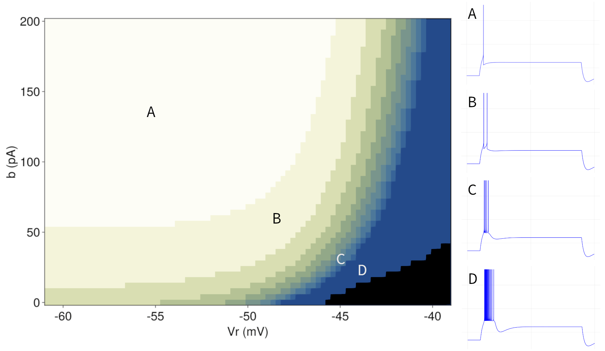
For the transient patterns, we are primarily interested in the number of spikes that the system generates before settling into a stable fixed point. A necessary condition for transient behavior is a high subthreshold adaptation (\(a = 8nS \)). As before, the adaptation time constant is set to \(τ_{ω} = 100ms \). Figure 8 shows the simulation results with respect to the number of spikes produced by a transient pattern. The results are consistent with the observations in the previous section. The spiking activity stops when a landing point falls into the basin of attraction of the stable fixed point (cf. Figure 5). For a lower reset value \(V_{r} \), there is only a narrow space below the fixed point for the system not yet to converge. Hence, in order to observe more than one spike, small values of \(b \) are required. Increasing \(V_{r} \) widens this space and we can observe bursts even with higher values of \(b \).
Figure 8: Left: Parameter space for transient patterns with the number of spikes as a function of the reset parameters \(V_{r} \) and \(b \). All other model parameters are fixed as described in section 3.3. The color gradient indicates the number of spikes from light (one spike) to dark blue (more than 10 spikes). Black indicates tonic spikes over the entire period of current injection. Right: Example patterns corresponding to the respective labels in the parameter space.
4. Implementation
We implemented the AdEx model using the Julia programming language and made the code publicly available4. Although working examples of various neuron models were already available5 in DifferentialEquations.jl (Rackauckas & Nie, 2017), to our knowledge there was no implementation of the AdEx model using this framework, and no example that successfully incorporated physical units. We implemented physical units with Unitful.jl.
We benchmarked our implementations and compared them with the Python framework brian2 (Stimberg et al., 2019). We used identical parameter sets and measured the runtimes for the Euler method with the identical fixed time-stepping. In all cases, the Julia implementation (with physical units) outperformed the brian2 reference implementation6. Moreover, Julia's state-of-the-art adaptive solvers appear to be well-suited for simulating neuronal activity. However, using adaptive time-step solvers can be challenging due to the AdEx model's exponential nonlinearity, but this discussion is beyond the scope of this paper.
If the reader is familiar with the brian2 framework, full implementations of the AdEx model are available in the framework's documentation. In particular, examples are available for the original paper7 (Brette & Gerstner, 2005) and the firing patterns paper8 (Naud et al., 2008).
5. Discussion
In section 2, we derived and motivated the AdEx model as an evolution from different integrate-and-fire-type models. As a result, the AdEx model is able to reproduce many electrophysiological features of real neurons. The wide range of firing patterns makes it a more versatile candidate compared to the LIF or EIF models. Moreover, both the LIF and EIF models are special cases9 of the AdEx model. The Izhikevich model shares many features with the AdEx model in that both models have similar bifurcation patterns, can be parameterized to have a wide range of firing patterns, and yet are relatively easy to simulate computationally. However, in particular the subthreshold behavior of the AdEx model is more biophysically realistic compared to the Izhikevich model, as it aligns better with experimental data (Badel et al., 2008). An intuitive reason is that the exponential nonlinearity better captures the dynamics underlying the sodium current, in particular the activation of sodium channels.
In section 3, we discussed how the AdEx model’s dynamics give rise to different firing patterns, such as tonic, adapting, bursting, transient or irregular firing. Important parameters are the adaptation parameters \(a \) and \(τ_{ω} \), the reset parameters \(b \) and \(V_{r} \), the spike threshold \(V_{T} \). For the parameter space, we were able to show that for a suitable set of adaptation parameters, the type of firing pattern depends only on the reset parameters.
In section 4, we briefly discussed our implementation of the AdEx model within the Julia programming language and conclude that the chosen environment is well-suited for simulating neuronal activity.
To summarize, while maintaining its simplicity as a two-dimensional dynamical system, the AdEx model is able to produce a broad spectrum of firing patterns and allows for a high degree of biophysical realism. It is therefore well-suited to analyze experimental data, simulate large spiking neural networks, and investigate questions in neuroscience related to neural coding, memory, and network dynamics.
References
Abbott, L. (1999). Lapicque’s introduction of the integrate-and-fire model neuron (1907). Brain Research
Bulletin, 50 (5-6), 303–304. https://doi.org/10.1016/S0361-9230(99)00161-6.
Badel, L., Lefort, S., Brette, R., Petersen, C. C. H., Gerstner, W., & Richardson, M. J. E. (2008). Dynamic i-v curves are reliable predictors of naturalistic pyramidal-neuron voltage traces. Journal of Neurophysiology, 99 (2), 656–666. https://doi.org/10.1152/jn.01107.2007.
Bezanson, J., Edelman, A., Karpinski, S., & Shah, V. B. (2017). Julia: A fresh approach to numerical computing. SIAM Review, 59 (1), 65–98. https://doi.org/10.1137/141000671.
Brette, R., & Gerstner, W. (2005). Adaptive exponential integrate-and-fire model as an effective description of neuronal activity. Journal of Neurophysiology, 94 (5), 3637–3642. https://doi.org/10.1152/jn.00686.2005.
Fourcaud-Trocm´e, N., Hansel, D., van Vreeswijk, C., & Brunel, N. (2003). How spike generation mechanisms determine the neuronal response to fluctuating inputs. Journal of Neuroscience, 23 (37), 11628–11640. https://doi.org/10.1523/JNEUROSCI.23-37-11628.2003.
Gerstner, W., Kistler, W. M., Naud, R., & Paninski, L. (2014). Neuronal dynamics: From single neurons to networks and models of cognition. Cambridge University Press. https://neuronaldynamics.epfl.ch/book.html.
Hodgkin, A. L., & Huxley, A. F. (1952). A quantitative description of membrane current and its application to conduction and excitation in nerve. The Journal of Physiology, 117 (4), 500–544. https://doi.org/10.1113/jphysiol.1952.sp004764.
Izhikevich, E. M. (2003). Simple model of spiking neurons. IEEE Transactions on Neural Networks, 14 (6), 1569–1572. https://doi.org/10.1109/TNN.2003.820440.
Izhikevich, E. M. (2007). Integrate-and-fire. In Dynamical systems in neuroscience: The geometry of excitability and bursting (pp. 268–269). MIT Press. https://www.izhikevich.org/publications/dsn.pdf.
Naud, R., Marcille, N., Clopath, C., & Gerstner, W. (2008). Firing patterns in the adaptive exponential integrate-and-fire model. Biological Cybernetics, 99, 335–347. https://doi.org/10.1007/s00422-008-0264-7.
Rackauckas, C., & Nie, Q. (2017). Differentialequations.jl – a performant and feature-rich ecosystem for solving differential equations in julia. Journal of Open Research Software, 5 (1), 15. https://doi.org/10.5334/jors.151.
Stimberg, M., Brette, R., & Goodman, D. F. (2019). Brian 2, an intuitive and efficient neural simulator. eLife, 8, e47314. https://doi.org/10.7554/eLife.47314.
Touboul, J. (2008). Bifurcation analysis of a general class of nonlinear integrate-and-fire neurons. SIAM Journal on Applied Mathematics, 68 (4), 1045–1079. https://doi.org/10.1137/070687268.
Touboul, J., & Brette, R. (2008). Dynamics and bifurcations of the adaptive exponential integrate-and-fire model. Biological Cybernetics, 99, 319–334. https://doi.org/10.1007/s00422-008-0267-4.
Christian Rohde
Personal Motivation
Learning about the foundations of biological mechanisms in the human brain, and gradually understanding how this contributes from one level of abstraction to the next, was my favorite part of the Cognitive Science Bachelor program. Thought this, together with some mathematical curiosity and passion for coding in general, I developed a keen interest in theoretical (or computational) neuroscience. The neurodynamics course and, in particular, the final project brought all these aspects together.
Good to know
Ideally, you are familiar with the basics of neuronal activity, especially the synchronization of neuronal population spiking. For example, you know that there are different frequency bands and different forms of cross-frequency coupling between neural oscillations. For an overview, see this paper.
Chemical signals are responsible for synaptic transmission involving neurotransmitters. The release of neurotransmitters into the synaptic cleft is usually triggered by an action or a graded potential.
The rheobase is the minimal current needed to initiate an action potential (when applied for an infinitely long time). The threshold potential (voltage) is the critical level that the membrane potential must reach to initiate an action potential.